CanalNetworkDocs

Longitudinal Route Design

Longitudinal design of routes is the stage where the engineer spends significant time working on individual canal routes, and exploring design scenarios. CanalNETWORK offers an interactive graphic environment with rich annotation to guide design process effectively.

Longitudinal design stage requires that the below workflow tasks are completed adequatedly:

1. Resolved network

2. Established network

3. Profile extracted

Once the above stages are complete, and data from each is accessible (See here for available ways to manage different data and make them accessible for CanalNETWORK), longitudinal profile design can continue.

Start Longitudinal Design

There are two ways to start the longitudinal design of a canal route:

1. In the plan view, zoom or pan to the desired roure, and left-click on it.

   Note: Right click does not load the profile data to the profile view axis.

   Note: Make sure the Multi-Select option is diabled, in Edit > Multi-Select or the toolbar button.

2. Press Ctrl+K or go to Workspace > Pick Route (AutoCAD),

Both options load and render longitudinal profile data, along with canal controls and flow profile information to the Profile view axis.

Note: The longitudinal design task follows a down-stream design approach, that is componenets of the route, including controls, drops, and segment assembly information, are positioned and designed from upstream end to downstream end.

The user can interact with the design as follows.

Adjust Control Inverts

Controls comprise key components in longitudinal design of routes. They represent acual control structures, such as Turn outs and division boxes. The primary task of the engineer can be to design the invert levels of these controls.

Note: Canal Controls, represented as vertical bars in the profile view axis, represent invert and hydraulic information at and upstream of the control location.

Controlling inverts and other hydraulic characteristics hosted by the control is possible from the Node Panel at the right side of the interface.

It is important to note that, all values displayed for a control node, are an exact copy of the design criteria, applied during canal sizing operation. Hence, any edit the user does for the control is effectively over-riding the provissions of the design criteria.

Select a control node in the profile view. Then:

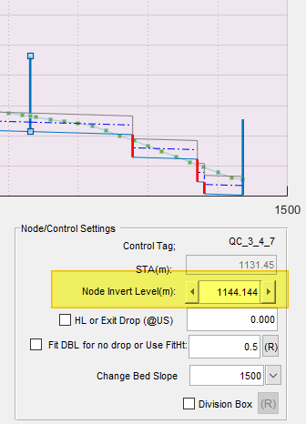
To change the invert level upstream of the control:

• Use Node Invert Level edit box to directly input elevation values

• Use the left < and right > arrow to increment the current value of the invert level for the control

Note: The algorithm maintains the settings in the design criteria regardless of the the user inputs. Hence, there is a limit to how high or low the invert can be raised or lowered. For instance, any control can not be raised above the level that is maintained by the bed slope of the upstream canal section.

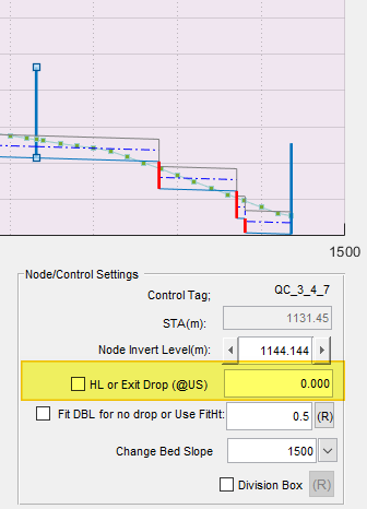
There are two ways to change invert level downstream of the control:

• Set Exit Drop: Type the desired value directly the Exit Drop edit box (with respect to upstream invert level.) Typically, this value is a negative value representing a drop in elevation calculated with respect to the upstream invert.

• Set Head Loss: Check the HL option box, and type a desired head loss value. This is also typically a negative value indicating the desired headloss to maintain as the flow transitions through the control. This process, calculates an exit drop at the control that can satisfy the desired head loss amount, and apply to the control.

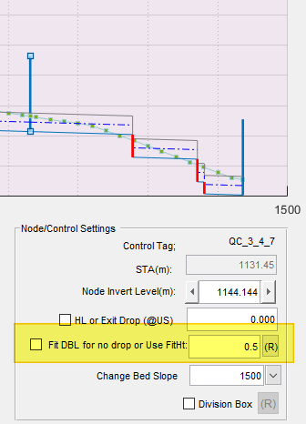
Change how drops are located upstream of the selected control, by:

• Change or set a fit height fitHt for drop positioning at Use Fit Height edit box. Drops are located in one of three ways:

  • fitHt <=0 ensures that drops are inserted where the bed level is exactly fitHt units below the OGL

  • fitHt >0 ensures that drops are inserted where the FSL level is exactly fitHt units above the OGL.

  • fitHt =-99 ensures that there is no drop inserted upstream of the current control.

• Check the Fit DBL for No Drop option to set fitHt to -99.

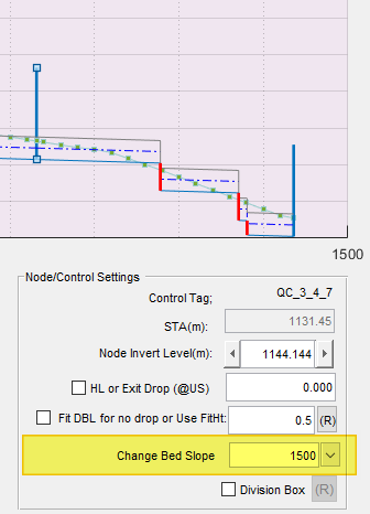
To Change the bed slope upstream of the control,

• edit the Change Bed Slope edit box to desired value. This is typicall a positive value equal to the desired canal slope (H:V).

• Click on the drop down menu at the right of the edit box, to pick from a set of default values.

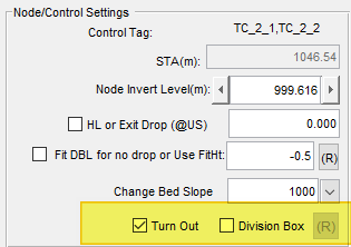
Finally, to change the functions of the control:

• By default, all controls are configured as Turnout structures. You can decide to change it to a division box struture or no structure at all. If HR/CR provissions are expected, then turning off both checkboxes ensure the control is treated as a simple junction (no structure associated to it). Such controls have no quantities associated with them.

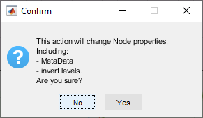
• To change the function of the control to a division box structure, check the Division Box option. (Note: Division boxes are allowed on Parent Canals whose capacity is <=80 litres per second.)

• This will throw the confirm dialog shown below.

  

• If user resonds with Yes button, then, this will invoke hydraulic calculation and design algorithm to size and position the control along with its branch canal(s) appropriately.

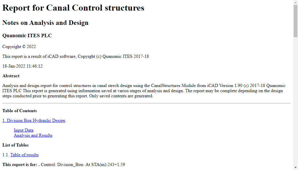
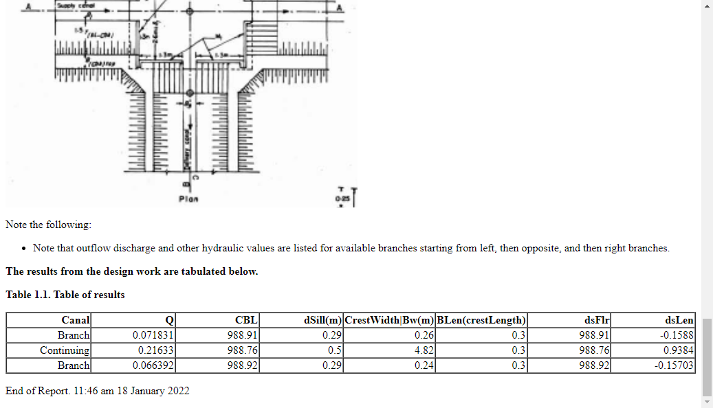
• One can view the results of the hydraulic analysis by clicking on the R button next to the Division box check box. A report of the following form will be generated informing the user of the hydraulic analysis carried out, and the adjustments made to the inverts of the offtaking canals.

  

  

• The same button also redesigns the division box currently selected, for any changes that may have been made to invert levels, flow depths, or similar. A new report, and a new set of invert levels are calculated and applied to the offtaking canals corresponding to the modification made.

To reapply the default criteria set for the entire route, thereby removing any and all overrides done manually, the user must resize the canal. See part of this guide on Design Criteria creation and use for more details.

Adjust Drops

Drops are created automatically following the variation of the ground level. They are positioned strictly per the provisions of CBL_designSettings parameter set in the design criteria. See Design Criteria Creation and Use for the meaning and use of each of these variables.

For many reasons, the automated design output will not satisfy the engineers desires. Each drop can be edited and adjusted as follows:

To change the location of the drop:

• Click on the desired drop. An interactive tool appears reading station location for the new locatio of the drop. Click at the desired new location, and the drop is repositioned to a new station.

Annotation information can also be used to guide drop insertion. Often times, one may want to locate the position of drops manually based on FSL-OG or CTL-OGL values. This can be achieved by using the above same method, but after invoking supported annotations.

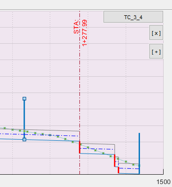
In the example below, the drop near statio 1600 is automatically positioned using the setting of FitHt=-0.5.This can be confirmed by starting the relevant annotator from Explore Solutions > Annotators > CBL-OGL. It can be seen in the annotator, CBL-OGL= -0.513, slightly higher than specified because of the position the reading is taken.

Assume, it is required to move this drop to a location where CBL-OGL is about -0.20. First, move the drop further right to about station 1+670.

Now, click on the drop again. The interactive, marker tracks the value of CBL-OGL as you move the location. Drag to the new location where CBL-OGL meets the desired value. In this case it is near station 1+639. Click, and the drop is positioned.

As shown below, there are other ways to edit drop positions. To manually change the location and/or height of the drop:

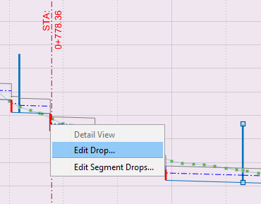
• right click on the desired drop, and choose Adjust Drop conext menu item. This will start a dialog box.

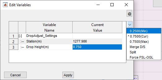
• Enter the desired station, and click on Apply. The drop is repositioned accordingly.

• Enter a desired drop height, and click apply. The drop height us adjusted accordingly.

Note: User inputs are guided by allowable values for the specific drop.

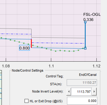
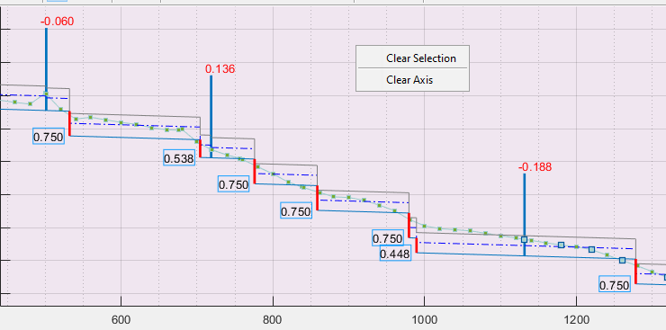
Some times the last drop inserted in a canal segment can have odd values (not suitable for construction.) In such cases the user can make fine adjustment by typing in numeric expressions in the Edit Node Invert edit box inside the Node Panel.

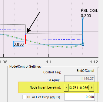
In above snapshot, the drop height of 0.836 can be adjusted to 0.800 by adding 0.036 to the invert level of the downstream control. The result is shown below.

Invalid Drop Locations

In rare instances, the sum effect of the drop location parameters specified by the user is not actionable. As a result, it may not be straight forward to position some drops. Also, the Explore Drops command may not collect and report drops in such segments.

In the above instance, the user wanted to adjust the first drop, and left-cliked on it. The Auto-Locator moves to an invalid station reading. This is often the case when working with short length segments, common to the first segment of all distributary canals.

Upon clicking (to accept the new location), the Invalid Input dialog appears, with recommendation to change values in CBL_designSettings. The corresponding setting for this particular instance are as follows:

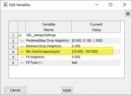
It can be seen that, the drop can only be located before the first control when attempting to maintain Min. Control Spacing settings. This is because, the set minimum control spacing of 15 meters can not be achieved in the current segment. Note the distance between the contols is 17m. To accomodate a drop, a segment length of 25m (5+15+5) is required, that is not available.

There are two ways to resolve this issue:

(1) Increase the segment length available: this must be avoided, because it entials chaning the layout design to create more space between the controls.

(2). Change the allowbale minimum distance between controls (as shown in row 4 of above figure.) Changing the first value to 2.5m for instance (i.e, dictating to observe only 2.5meters between controls) allows to re-position the drop feasibly in the segment range.

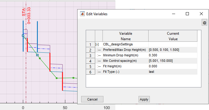
Note: The minimum acceptable spacing between structures is sligthly greater than 5.0meters. In line with this, it is strongly recommended that the available distance between any two controls in the network is at least 20meters.

Provide predefined list of drops

Once can also override the entire list of drop heights and their stations in a canal segment, to replace with own predefined list. This may be particularly helpful when modeling existing projects.

To do this:

1. Right click on any one drop of the desired segment, and choose Edit Segment Drops.... This will invoke the drop adjust dialog.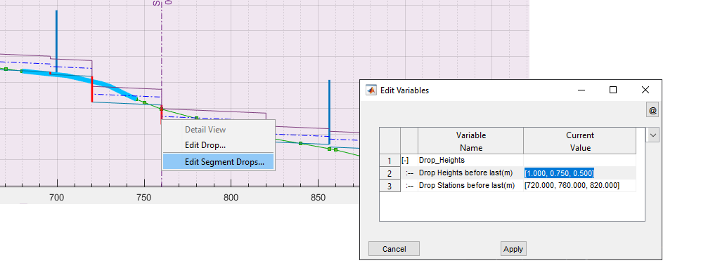

   

2. Input the drop heights in the first row, and thier stations in the second row.

3. Hit Apply when done.

This will create a new CBLinformation for the segment that accomodates the prescribed drop heights and locations.

Note: The invert of the control at the downstream end of the segment will adjust automatically to a corresponding elevation.

Note: There are no limits to the size of the data length to be provided for such prescrptions. However, both the height and locaiotn data must be of the same length, and respect the data input expectations. Otherwise, the action will not take effect.

Adjust Canal Assembly for Segments

The last area of control for the user to guide and influence longitudinal canal is the Canal Assembly panel. In this panel, information regarding the parameters that determine the shape and size of the canal section and its flow parameters can be adjusted.

Note: When a node is selected, this panel shows flow information in the segment upstream of the control. The small rectangular button, also known as Perfoamnce Indicator button, show the acceptability of the flow conditions. A red color indicates tells that either the velocity limits or the shear stress limits are not respected, and redesign is needed.

The user can interact with the canal assembly informaiton in many ways. Select ((click on the OGL profile line) a canal segment or reach in the profile view that you want to edit and follow below guideline:

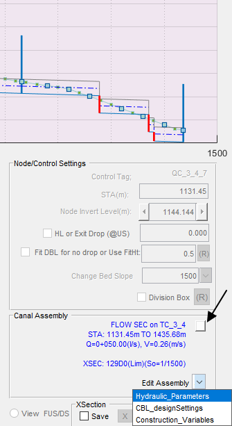
To change the flow section, drop design or construction parameters:

• click on Edit Assembly drop down menu, and choose the relevant design option. This will open up a dialog to edit corresponding variables fot the canal segment. See Design Criteria Setting and Use for details on each variable and their design implication.

To redesign the flow section by adjusting the slope within allowable performance criteria:

• Click on the Perfoamcne Indicator button. This will invoke a dedicated interface to interactively design the section.

• After making the desired changes, close the interface. The user will be promted to apply the changes, and the profile view will update automatically to update the changes.

• See further below topic Solving Optimal flow sections for Individual segments further below for guidance on using the solve function.

Update Segment Data

Information for hydraulic and formation design in segments may require updating from time to time. Typically, a segment may exhibit a behaviour that is not expected as below:

• Variation in exit level

• Non-conformance with OGL and (beg/end) control inverts

The below picures demonstrates one such instance. Here, the control level and the CBL level at the control do not much. In this particular instance, it resulted from adjusting drop heights for the specific segment.

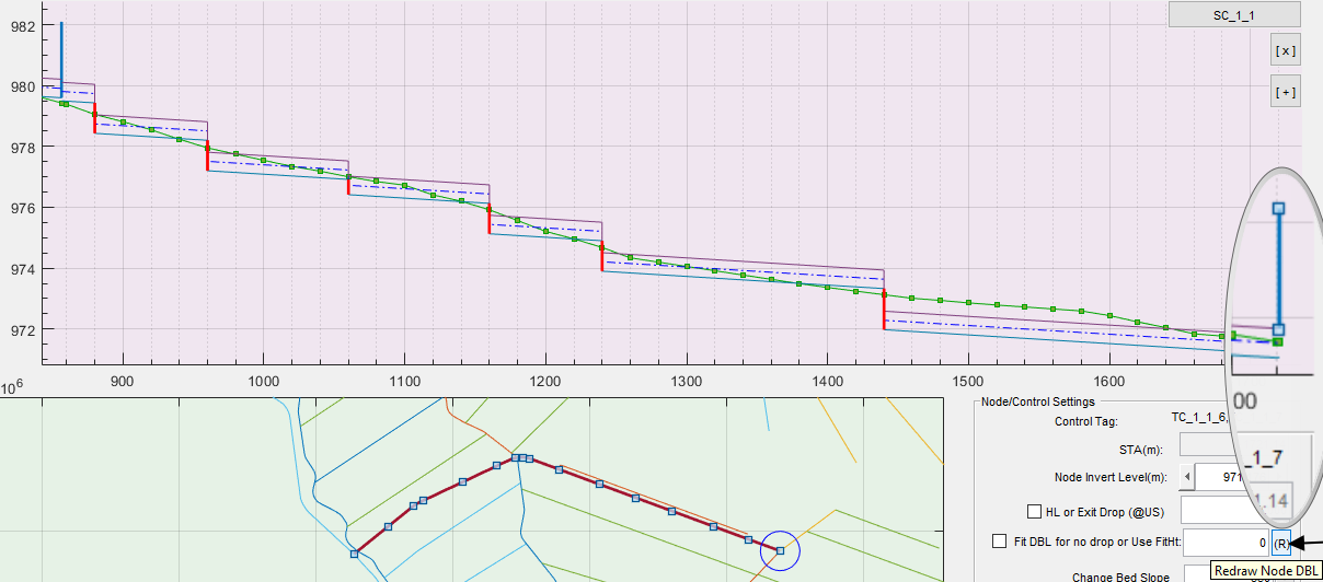
To resolve these issues, DO NOT USE ReDraw Node DBL button, as shown at bottom right. This will erase all drop station and heigh information, and create a new data set. Instead, refresh the profile view by clicking the canal route in plan view.

Note: ReDraw Nod DBL button, resets ALL drop information (i.e. station and fall heights) to null, and re-create them based on automatic settings. Beware, that this action, aslo does the same for the immediate downstream segment (if any). Use this button with descrition.

In above note, you notice that the reDraw button also creates an auto-generated data set for drop location in the immediate-next segment of the control. This is mandatory process, to ensure that any changes in invert level of the control node, is accomodated with respect to the downstream setment.

Using Floating Nodes

Floating nodes are nodes (or contols) similar to other nodes, but can be used to represent different hydraulic and physical constraints along a canal route. They can be an effective way to regulate and interact with the longitudinal design of a route. The following notes deal with the insertion, specification and management of floating nodes to emualte practical design considerations.

Inserting a floating Node

Floating node parameters

Deleteing a floating Node

Canal Structures

Special Segments

Exploring Solutions

There are multiple ways to explore and interact with the solutions of a longitudinal profile design of a canal route. These are all accessible from the menu Explore Solutions. These are categorized in to two groups, annotations and data tables.

Creating and Managing Annotations

Users can create and manage various annotations to keep track of the changes happening, as well as ensure key criteria are met.

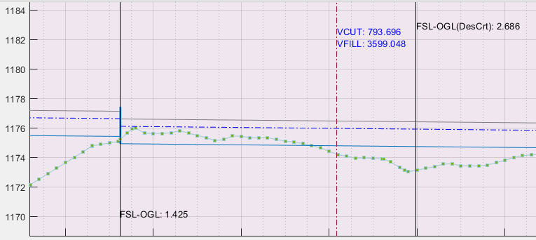
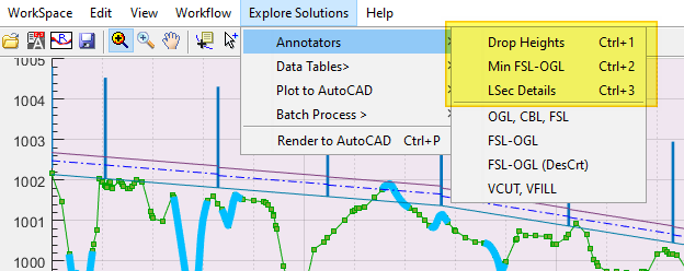
To show drop heights, FSL-OGL value at controls,

• Go to Explore Solutions > Annotations > Drop Heights to show drop heights for generated drops.

• Go to Explore Solutions > Annotators > min FSL-OGL to calculate FSL-OGL value at each control and render values by color in comparison with design criteria value.

To show hydraulic annotations such as OGL, CBL, FSL inforation:

• click on the appropriate annotator from Explore Solutions > Annotators and interactively position the cursor line. The results will be displayed.

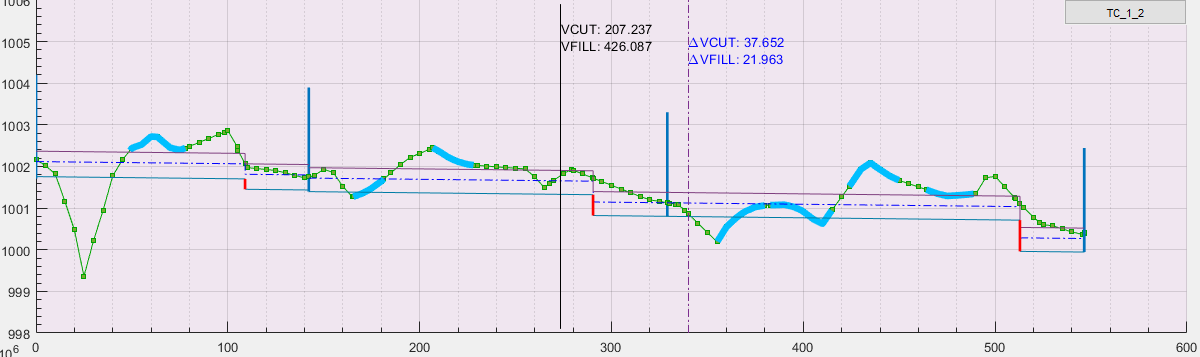
An other imporant annotation available is cut and fill volume annotator, shown above. This tool can cumulate volumes of earth work for entire reach or between selected stations giving an insight in to the cost of the design. To view volume informaiton:

• Click on Explore Solutions > Annotators > VCUT, VFIL menu item.

Note: If there are annotation markers in the profile view, then the partial volumes are automatically calculated and displayed. In such cases, all markers with in 100m of start and end station, or 100m distance between are ignored - i.e., do not affect the partial volumes calculated. The values are interpolated between succesive stations, and hence are accurate only at data stations.

Yet another helpful annotation is available from Explore Solutions > Annotatiors > LSec Details. This will display details of the longitudinal design including station range and flow section details for each segment of route. In addition it also annotates canal curve information if avaiilable.

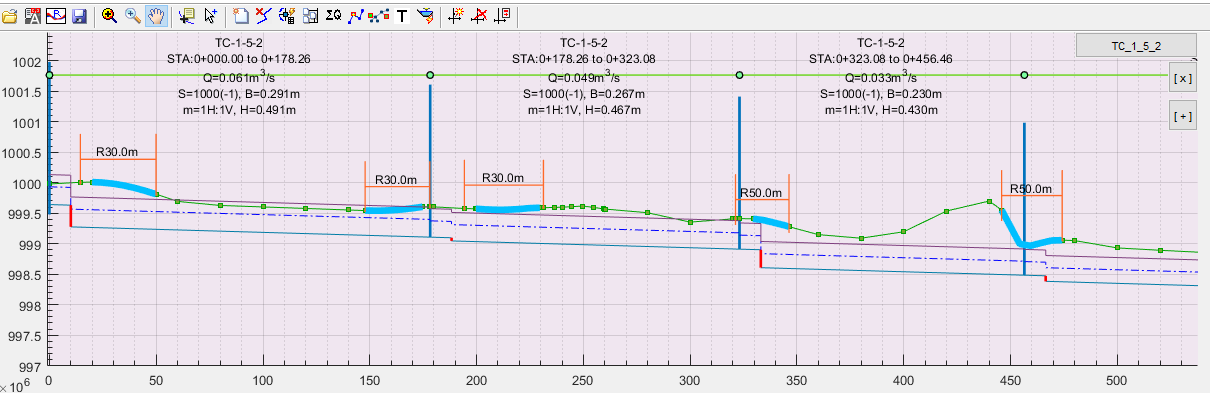
The above described annotations provide a quick and reliable overview of the hydraulic status of the canal. Some of the annotations also vary dynamically along with design changes by the user, to help decide whether design objectives are met.

Note: The above annotations can easily be accessed with the following short cuts.

Ctrl + 1: Display on/off drop heights

Ctrl+2: Display on/off Min FSL-OGL states at controls

Ctrl+3: Display on/off LSEc Details

Viewing and copying table data

The other group of tools to explore solutions is viewing tabular data. The solution for longitudinal design of routes incorporates tabular data. These are accessible from Explore Solutions > Data Tables. There are five table data available for viewing.

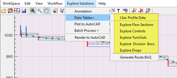
LSec Profile Data

This table shows extensive detail of profile data along with canal bed level and embankement formation data for the entire range of stations in the route.

Note: The data are tabulated at exactly the same incremental stations generated during profile extraction.

It is also important to note the following additional refinements, that are not specified by the user, rather applied in run-time.

(a) the data is further refined at additional stations, for:

• control locations, including floating nodes.

• Drop structure locations

(b) calculations in transverse direction depend on the offset data interval during profile extraction. However, additional refinements are applied to the transverse data set if:

• the number of offset locations is less than 5, and

• the applied refinement is -15:3:15 in conventional notation, or -15, -12, -9, -6, -3, 0, 3, 6, 9, 12, 15.

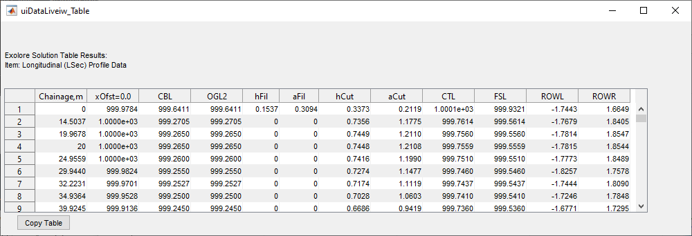
In the table:

Chainage: Station locations where data is extracted (See below note.)

**xOfst=0.0: ** OGL at centerline

**CBL: ** Canal Bed Level value at the station

**CBL2: ** Final excavation or fill level at a station, after considering canal lining thickness (if used.) If no canal lining is used, CBL and CBL2 contain the same values for a given station.

hFil: Height of fill caculated as CTL less OGL at centerline

hCut: Height of cut calculated as OGL less CBL2 at centerline

aFil, aCut: Area of fill and Cut work, respectively, at the particular station.

work at the par

CTL: Canal Top Level

FSL: Full Supply Level

ROWL, ROWR: End of fill or cut lines on ground surface measured from the centerline of the canal to the left, and to the right respectively.

You can copy the table using the Copy Table button at the bottom, and paste it to an other applicaiton such as MS Excel or Word, for further processing.

Note: The station listing in the data table is extended to include control and drop locations, in addition to the station marks specified during profile extraction stage.

The table headers are explained in below schematics.

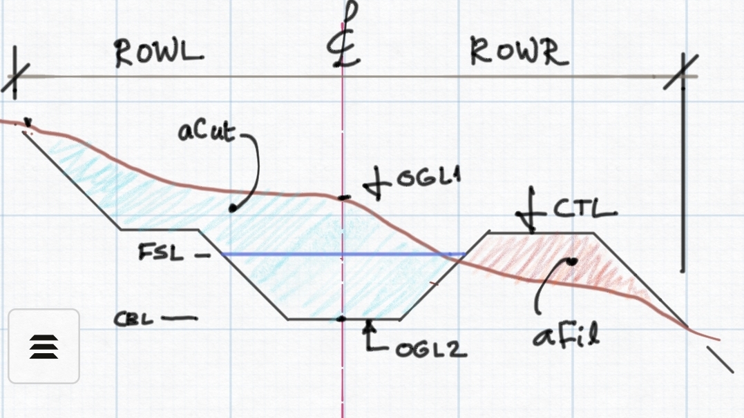
Schematic of a typical canal cross-section, showing details for unlined canal.

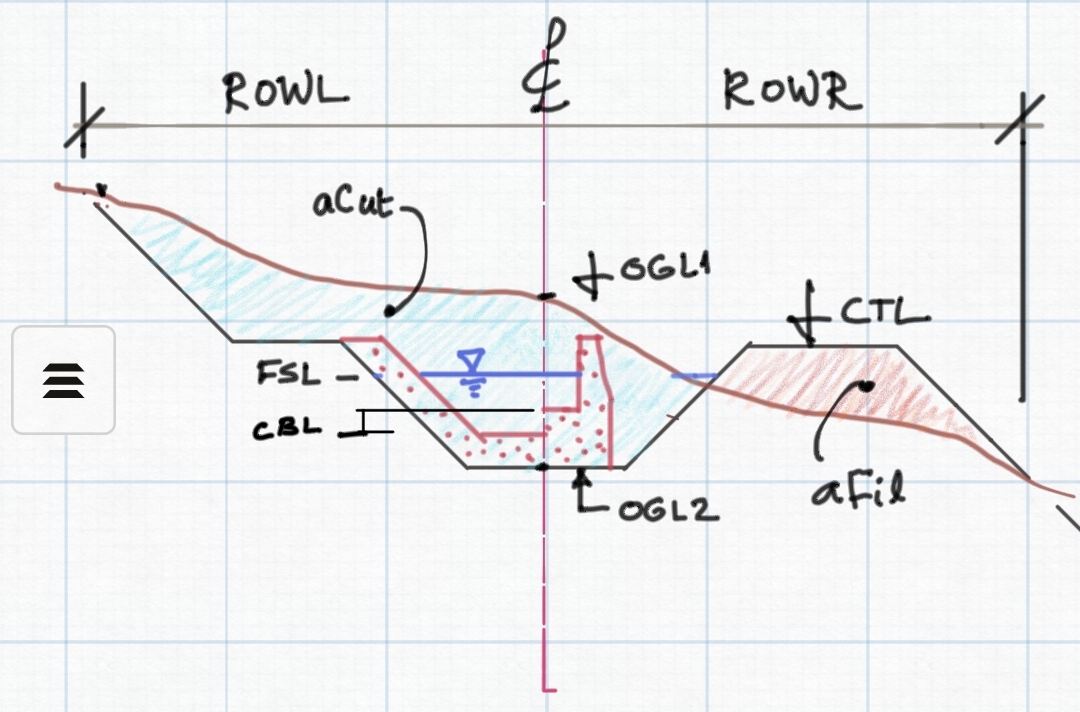
Schematics of a typical canal cross-section, showing details for thin (left) and Thick (right) lined canals.

aCut and aFil are determined by working out an exact analytical replica of the above geometric arrangement, and calaculting the area bounded in the corresponding regions. Typically, the analytical geometry is worked out for:

• a prevailing OGL (transverse profile)

• designed canal section geometry, such as bottom width, side slope and canal depth.

• superposed with values of Cut Shape and Fill Shape values input in construction variable settings, such as working space (in case of linings), berm width, cut/fill slopes and heights, number of berms, etc.

Hence, all results of the table can be considered an accurate representation of the built condition, given the transverse profile adequately represents the expected terrain variation at the particular station.

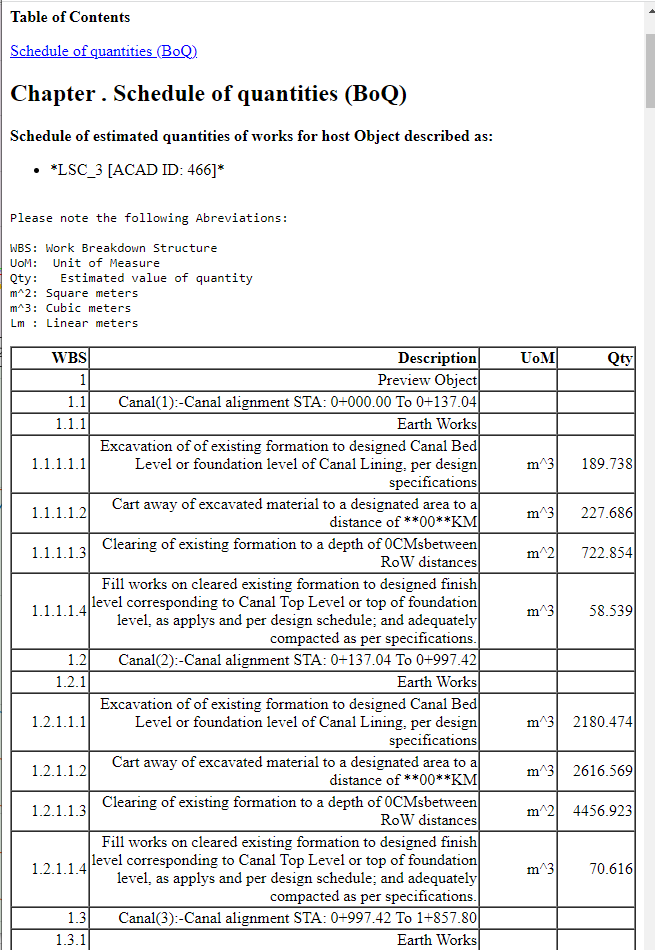
Bill of quantitiy estimates for earth works are estimated by cummulating areas of cut and fill at each succesive station, and applying the trapezoidal method. This method utilizes the approximation used for ‘numerical integration’, that breaks down areas in to trapezoids with more easily computable areas.

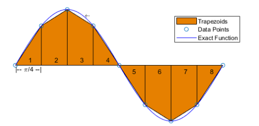
The trapezoidal method of volume estimation generalizes to:

where x1, x2,… xn represent the station locations for the corresponding aCut and aFil funtion values.

Note: Cart away volumes reported on BoQ table represent the total excavated/Cut volume multiplied with hardcoded loosness factor of 1.2.

See Design Production Section for more information ob BoQ estimation, and how clearing depth is considered.

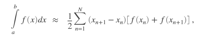
Exploring Flow Sections

This command generates the hydraulic design results for flow sections corresponding to each segment in the canal route.

In the table,

STA: Station range of the flow section

Q: Designed Dicharge capacity of the flow section, m3/sec

N: Manning’s roughness coeficient

FSD: Full supply depth, or Flow depth calculated by solving mannings equation.

FB: Freeboard used

So: Design bed slope

m: Side slope of the flow canal section

B: Designed Bottom Width of the canal seciton

B/D ratio: The ratio of bottom width to depth used to design the flow section

A, P, Hyd.R: Wetted Area, Perimeter, and Hydraulic Radius of the flow section for the above dimensinos

V: Flow velocity for the flow section

Vchzy: Chezy’s flow velocity calculated for the flow section

Vratio: Ratio of the two velocities calculated. ECSDWC design guideline recommends that that this ratio must be close to 1.

Taw: Calculated maximum anticipated shear stress for the flow section.

Flow sections can be generated to an AutoCAD environment as detailed drawings, by linking to iCAD’s CanalManning module.

Also:

V: represents actual flow velocity in the canal section

Vchzy: Chezy’s flow velocity in the canal section, estimated from:

v= c x (R/So)^(-1/2), and

c= NxR^(-1/6)

Vcr: Criteria velocity estimated from:

Vcrt= 0.546*y^0.64

Vratio: Velocity ratio determined from

Vratio= Vchzy/Vcrt

Some practitioners recommend to accept design sections whose value for velocity ratio is close to unity.

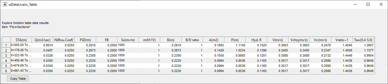
Exploring Controls

This menu command generates a list of all the controls in the canal route, that define the connection between succesive segments, as well as junction with brnach canals - if any.

In the table, the following defintions apply to the terms listed:

Type: The function of the control, set to either Turnout or Division box.

US Invert: the invert level, or the CBL, just upstream of the control location.

DS Invert: the invert level, or CBL, just downstream of the control location. This accounts for any Exit Drop Height specified for the control - if any.

Fall Height: The difference between US and DS invert levels

FSD: Flow depth for the flow section corresponding to the segment upstream of the control location, and

FSL: the full supply level just before the control location.

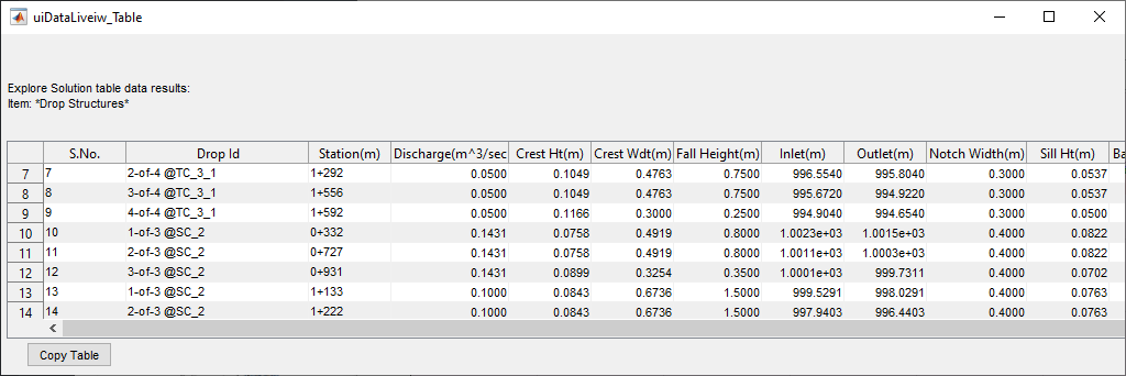
Exploring Drops

Similar to above commands, this command list all the vertical fall structures for the route.

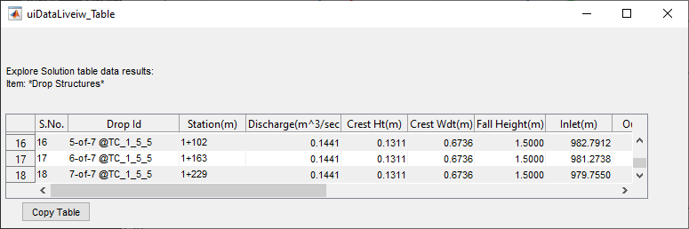
The table contains a rather long list of parameters for each drop:

Station: Location of the drop structure

Discharge: The design flow capacity of the drop passing through the structure.

Crest Ht: The height of the over flow crest above the US Invert level for the drop.

Crest Width: The width of the drop structure just before the overflow span at the crest, also extending to the stilling basin compartment.

Fall Height: The elevation difference between the US (Inlet) and DS(Outlet) invert level of the drop, as defined below.

Inlet, Outlet: the invert level, or CBL, just upstream and DS of the drop location, respectively.

Notch WIdth: The width of the overflow section just at the crest.

Sill Height: The height of the end sill provided for the drop, just before joining the continuing (downstream) canal reach

Basin Length, WIdth: The length, and width of the stilling basin to be provided

Basin Thk: The thikness of impervious floor to be provided under the stilling basin to ensure safety against excessive uplift pressure. (this is dertermined assuming massonry material with a unit weight of 22KN/m3)

US, DS Cutoff: Depth of cutoff wall provided at begining and exit of the drop structure.

Protection Length: Recommended length of protection layer to be provided both upstream and downstream of the drop structure.

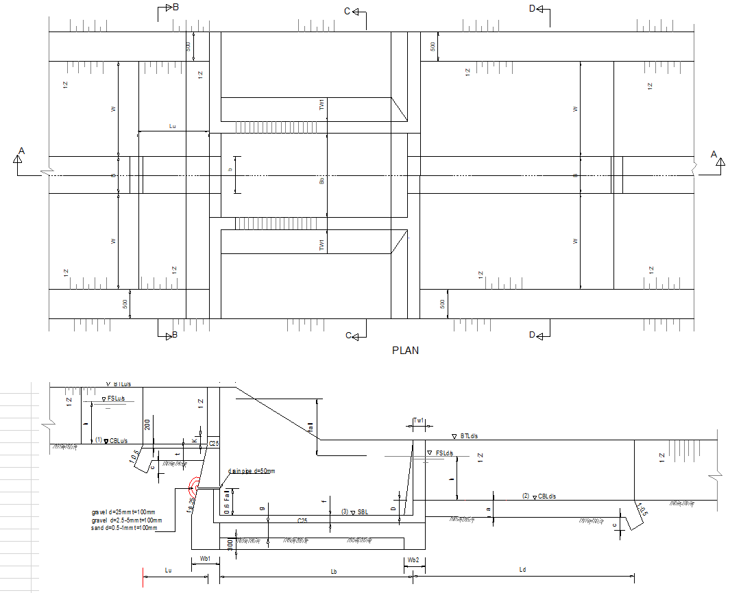
Figure: Details of a Drop Structure from ECDSWC, and some of dimensions included in the standard output of Explore command.

It is possible to extract the drops of a number of canal routes in one go. To do this, select all the routes whose drop list is desired, and invoke the command Explore Solutions > Data Tables > Explore Drops.

Exploring Turnouts

This option specifically lists the relevant construction dimensions for each turnout structure found on the route.

The symbols for the dimensions are explained in the accompanying drawing below.

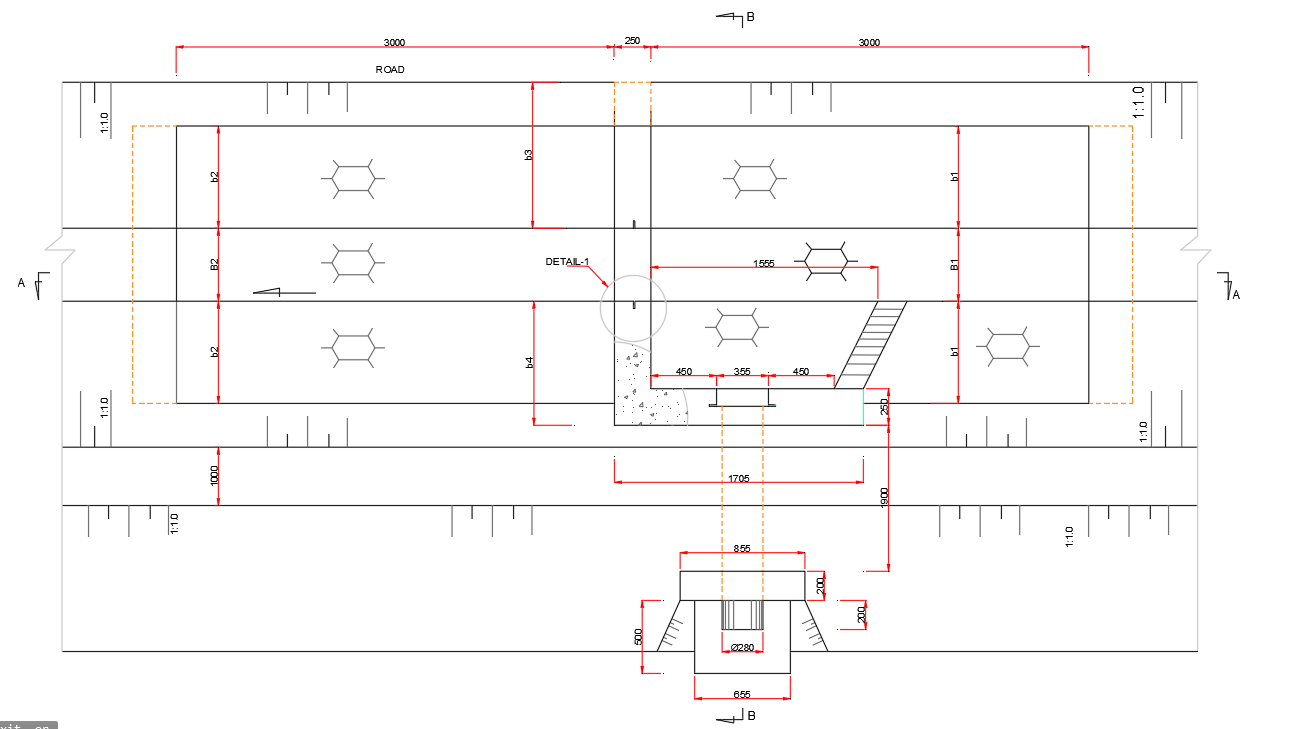
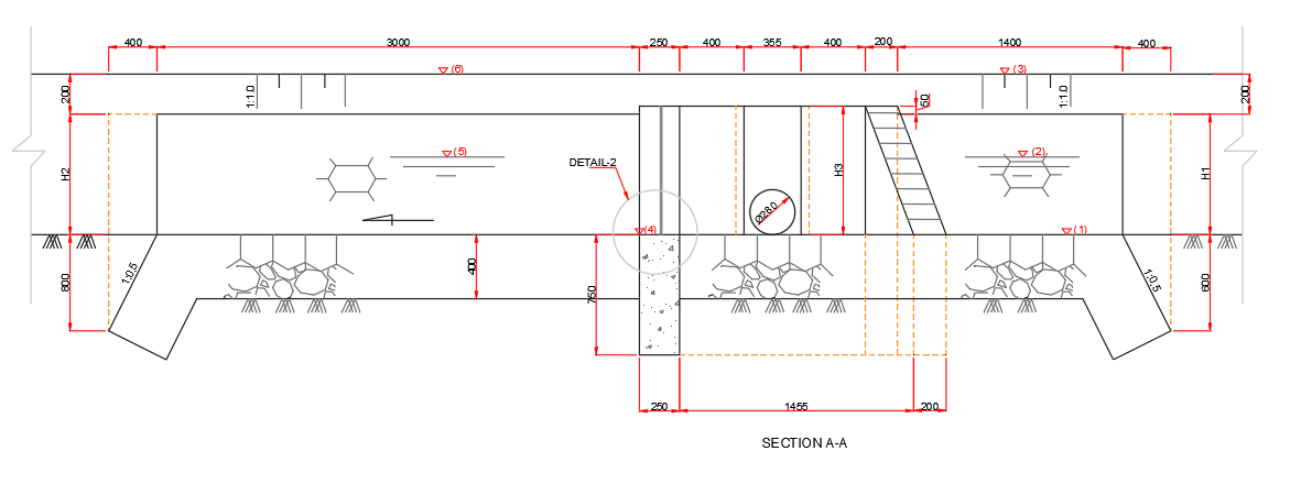
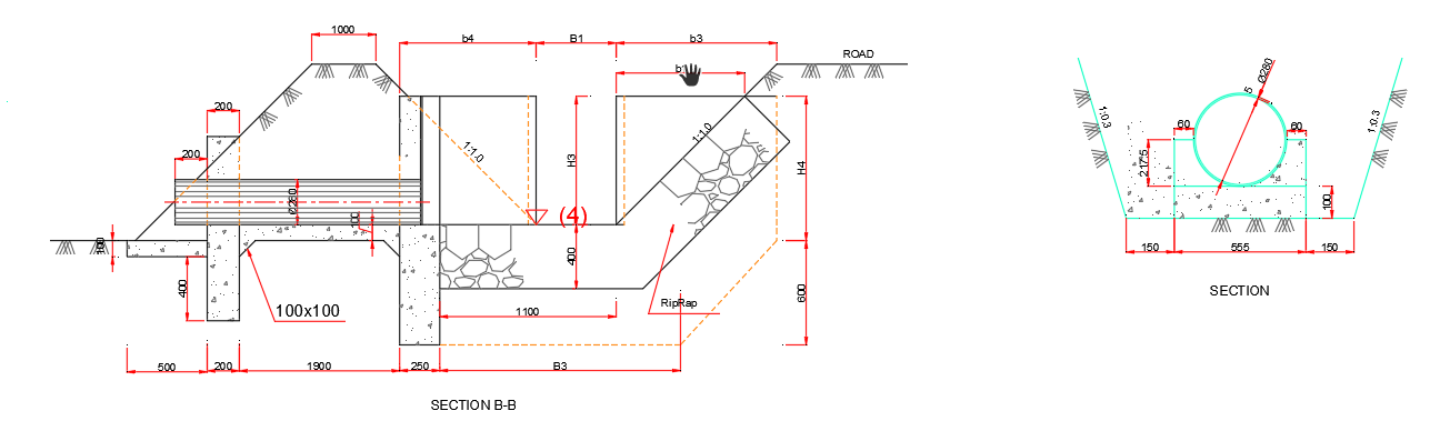
Figure: Tunrout Structure detail drawings from ECDSWC, with dimension detail corresponding to the symbols in the explore output table.

**Notes on BoQ calculation for Turnouts**

The calculation of quantity items for turnout structures is based on the sizes of the canals involved, and some fixed parameters in the reference resource. The following are key paramters used, also indicated in the drawing above.:

• Thickness of lining and cutoff walls (upstream and downstream) set to 0.40m

• Thickness of notch wall is set to 0.25m

• The depth of cut for earth excavation calculation is calculated from:

• dFloor= OGL at control location (centerline) - lowest excavation level, where lowest excavation level is estimated from bed level of lowest canal bed (upstream od downstream, especially for turnouts with falls), less 0.40m thickness of bed lining, less compacted backfill height provided in Control_BoQSettings (under network preferences).

The cut volume is calculated using:

• dFloor

• Ltotal=6.0m

• BTotal=2*(THK + b1) + B1;

• Working space, and m values from control_boqSettings

Thus:

Vcut= dFloor x (LTotal+mxdFloor) x (BTotal + mxdFloor)

Note: Tunrouts can be combined with drops. If controls for Turnout locations have drops, the stilling basing structure will be sized and provided similar to the design approach for othe drops. The results are included in BoQ quantity. This functionality is not applicable to Floating Nodes or Division Boxes.

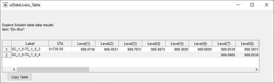
Exploring Division Boxes

Similar to turnouts, this command specifically lists the relevant contruction dimensions for each division box structure found on the route.

The symbols for each dimension heading is described in the below drawing.

Fig: Drawing for a typical division box from CDSWC, showing the deginition of symbols used in the table listing.

Viewing BoQ data for a route

After the above solutions are explored, a complete BoQ information can be generated for a route as follows.

1. Start the command from Explore Solutions > Data Tables > Generate Route BoQ.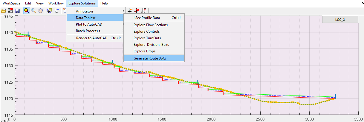

   

2. This will extract all available informations, and request output specifications.

   

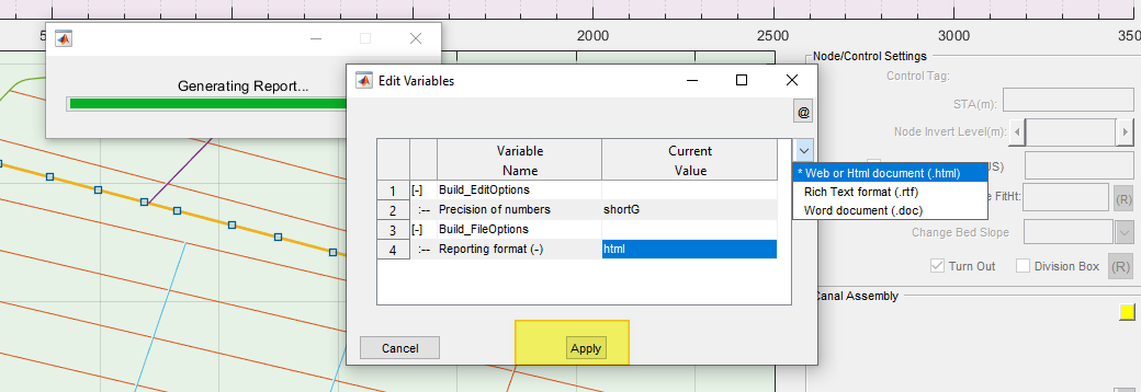
3. The report is generated per specified output format.

   

Note: If all solutions are not explored, generated BoQ may not be complete, or not succesfully reported at all.

More detail is available under the Topic Design Production.

Batch Explore of Solutions

Exploring solutions is desired to analyze and confirm the outputs are acceptable, or if there are modifications required to the design. It is also important for production tasks. However, it can be tedious to run all the above commands for each canal in a network of canal systems. To assist in this process, batch processing options are available. This allows to automatically run the solutions for a number of canals at a time, and update the data contents for each route.

To use this tool, to explore solutions for sub canals of a route:

1. Select the parent canal in layout view. In the figure below, a secondary canal is selected.

   Start the command from Explore Solutions > Batch Process > Batch Explore SubRoutes...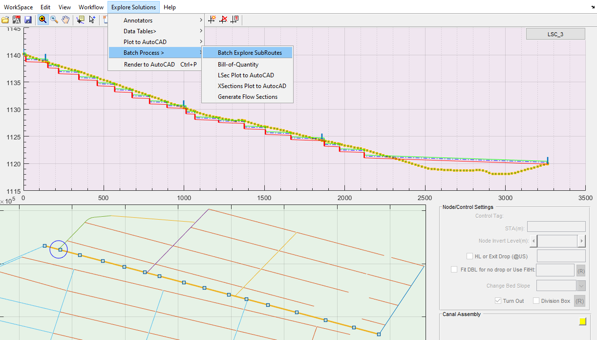

   

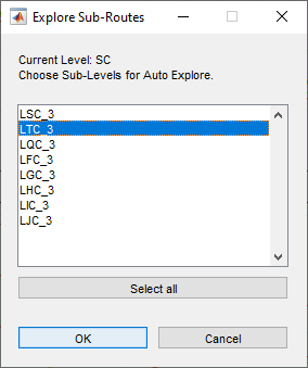
2. Choose the level or generation of canals whose solution is desired, from the dialog below. The immediate generation TC is selected in this case.

   

   Your choice is confirmed in the dialog displayed. Confirm action by clicking on Go button.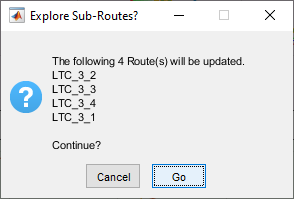

   

   This will run each of the branch canals for the above list of solutions, namely - Lsec profile data, drops, turnouts and divisionboxes. In the process BoQ data is updated and stored.

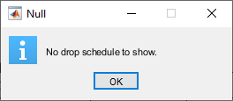
   When no components are found on a given route, the following dialog appears to provide the information.

   

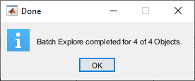
3. Once all routes in the specified generation are complted, the completion dialog shown below is displayed.

   

Creating and Viewing Cross-section views

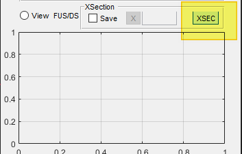
One can easily view the cross-section at any station along the canal route. To view cross-sections, make sure the desired route is selected in plan view, and its details are presented in profile view. Then:

Toggle on the XSEC button near the detail view area.

if the Lsec data is not created yet, the following message is thrown.

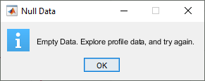
Create the data from Explore Solutions > Data Tables > LSec Profile Data. Then try again.

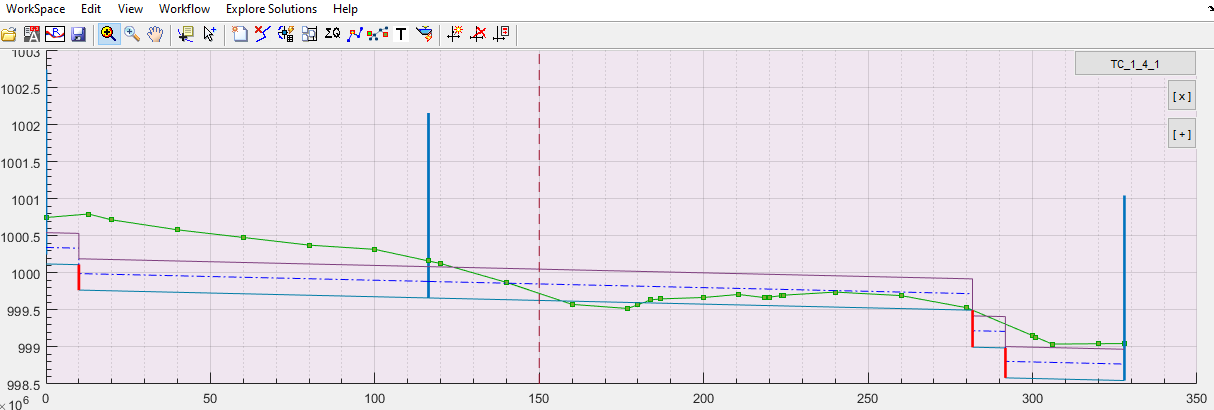
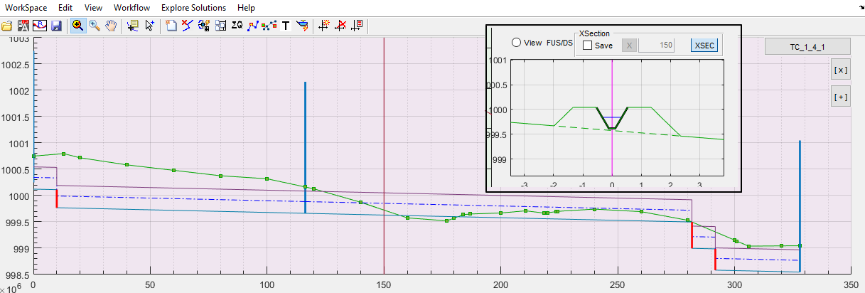
A vertical broken line is created at station 150 by default on the profile view. Click on the line to generate the cross-section on that station. The line will change to a solid line, and the cross-section is displayed.

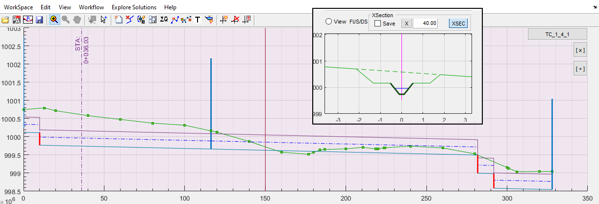
To view cross-sections at other stations, click onthe solid line. An interactive location bar will be displayed. Click on any desired station, and the cross-section at the new location is generated.

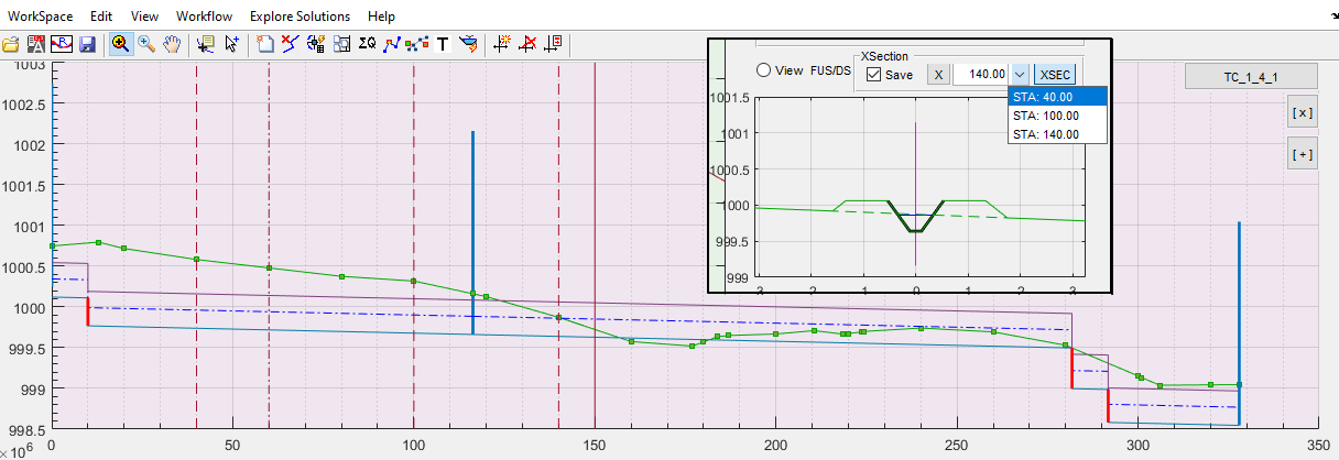
The stations viewed can be saved for latter use. To save selected stations, click on the Save check box on top of the detail view. This will make sure that every station picked is saved. Such saved stations are made availble any time when clicking on the route, and can be exported to AutoCAD.

Learn more about this on documentation for Design Production.

Copying table data and using in other applications

All the data presented in the form of a table can be used in other applications, e.g., report writing in MS Word or further data processing in MS Excel. The Copy Table button provided at the bottom of the table display interface just helps do that. To copy the data content of the table view interface, click on the button.

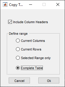
Choose your preference as shown above, and jit Ok. The data is copied to the Windows Clipboard. You can now paste the data to your desired application and use it.

Using Advanced tools for longitudinal design

AutoDesign

By default, the software generates a tentaive longitudinal profile for the route upon refreshing the profile view. Characteristics of this tentaive design include, bur are not limited to, the following:

• applies the set design slope from the design criteria for the specific route through out the reach

• automatically positions the invert levels of controls to ensure flow of water down stream. To this end, controls may be fixed for no drop structure upstream of the control location, or with drop structure depending on available gradient.

For many reasons, this tentative design will not meet operational requirements. For example, slope must vary depending on the ground level variation. Accordingly flow velocity varies. Further more minimum flow level above ground leve is often a strict requirement. This tentative design does not, however, account for this.

Auto Design tool implements a sophisticated algorithm to factor all the above requireemnts during design work. In the latest version, Auto Design tool is improved to complete longitudinal design of routes faster. The tool now generates the best achievable bed level profile for the given set of conditions to the route. The given set of conditions are as depicted in:

• design criteria provisions, most notably the following:

  • maximum and minumum allowable velocities,

  • allowable shear stress.

  • allowable minimum FSL above OGL

• variation of ground level in the entire reach of the route

Once again, the careful selection and setting of design criteria for canal routes can not be overemphasized. It affects the outputs of the automatic design, and hence directly impacts the time an engineer spends to complete the design of a single route.

Solving for optimal flow section for individual segments

Flow sections for individual segments, and the wider network of canals in general, are often expected to perform under established constraints that include:

• minimum non-silting velocity

• maximum non-scouring velocity

• Maximum allowable shear stress

The flow section design tool offers the capabilty to interactively vary the bed slope of a given canal segment and see impacts on above parameters. The accepted design detail can be applied to the segment at the end.

This tool is availiable for a single segment in the profile view, and accesible from the Indicator Button in the Assembly Pannel pannel.

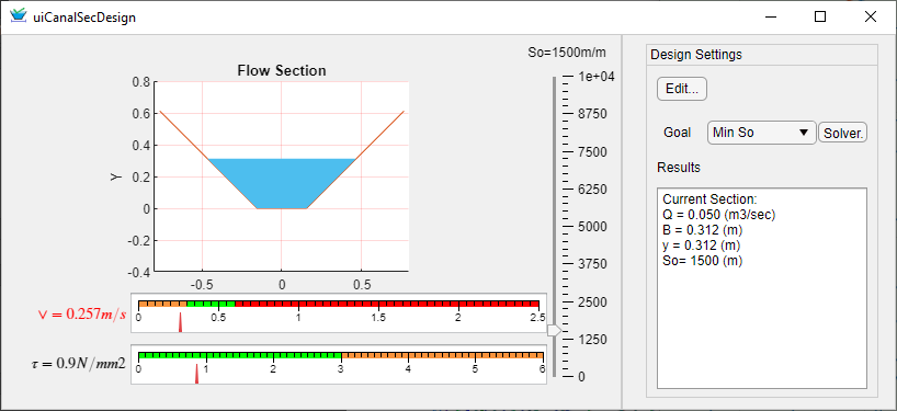
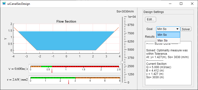
To start it, select a desired segment from the profile view. The Performance Indicator Button will be active. Click on it. The Canal Section Design interface will pop up.

Note: this interface starts with the hydraulic design parameters for the selected segement, and no data entry is required.

The main purpose of this interface, among others, may be to anlyze the variation of the flow section as the slope varies. As the slope is varied, by dragging the vertical bar the flow section and corresponding flow velocity and sheat stress developed are computed and displayed. The colored scales on the gauge bars provide feedback on appropriateness of the slope.

To see how performance of the canal varies:

• change the slope by clicking on (or draging the marker) on the vertical slider bar representing the bed slope of the canal. The flow section, the resulting velocity and shear stress values change accordingly.

• The updated flow section is drawn, and also the details written to the Results area on the right of the interface.

The Solver function offers a convenient and automatic tool to determine the best fitting slope that respects the constraints for limiting velocity and shear stress set in the design criteria.

• To find the minimum slope possible, change the Goal setting to Min So, and hit Solve…

• To find the maximum slope possible, change the Goal setting to Max So, and hit Solve…

In both cases, the results are generated accordingly.

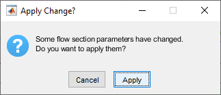
Upon satisfactory design, close the dialog, and accept the Apply request in the dialog that appears.

Note, the following limitations apply:

• Minimum calculated slope can not be lower than 50 (50H: 1V)

• Maximum calculated slope can not be higher than 10,000 (10000H: 1V)

AutoDesign for Route

The above procedure used for designing a single segment of a given route can be applied for an entire length of a route. To do so

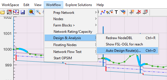
• Go to Workflow > Design and Analysis > Auto Design Current Route

• The process will continue in the background (with out invoking the Canal Section Design interface), but applying the changes to the segments.

Note the following added functionalities in this use-case:

1. Automatically considers the available slope from the OGL. Note here that the ground slope is calculated from invert levels of the upstream and downstream nodes of each segment, and hence assumed to be straight line.

2. Automatic positioning of inverts attempting to respect minimum FSL-OGL value in the design criteria set, where possible.

To see the viability of the result from this auto-design process, the user can create and manage annotations - especially:

• Drop heights: looking out for non-standard drops that may have been created, and adjusting if necessary. (see below Design Aids Available for Completing Design of Routes below.)

• minFSL-OGL: looking out for red-colored texts, indicating the desired criteria value is not met on those controls, and adjusting the inverts manually if needed. (See Adjust Control Inverts above.)

Override design criteria (Exception)

Canal routes, every time they are refreshed, refer to the design criteria corresponding to their level or generation. To override some of these parameters as the site condition may require, users have to change junction node and canal segment assembly criteria. This makes the job time consuming, particularly for long canal routes.

Instead, users can over ride the entire design criteria for a canal route and allow specific criteria for a route.

To set override values and apply to the current route:

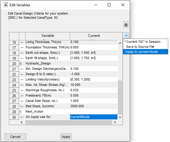
• Start the editror from Workspace > Manage Design Criteria > Set Edit Design Criteria…

• Change the values of the desired parameters

• Go to the final row, and for the On Apply Use for choose Current Route.

• Hit Apply to complete. This will review every aspect of the route to conform to the new set of criteria.

Note: The new set of criteria are also saved on to the exception data string for the route. This allows to re-visit the input data at a latter stage, and modify it. If not needed, it can be removed from Edit > Route Exception > Manage Exceptions...

Important: Exception design criteria EXCLUDE all variables in the command criteria group of variables.

AutoDesigning a Selection of Routes

AutoDesign tool can be applied to a selection of routes in one go. To start the tool:

• Select the desired routes in the plan view (iwth Multi-select mode set to ON). Use available tools from Edit > Select Routes if needed.

• Go to Workflow > Design and Analaysis > AutoDesign Route(s)...

This will start the process for all selected routes sequentially.

Important: It is important to revisit the designs for each route designed with the Auto tool, and make any adjustments before production.

Note: AutoDesign task can not be undone. To reset to original tentative settings, select the route, apply Resize. Design parameters are reapplied. To view the updated view, click on the route in plan view, which will refresh the view in Profile View Axis.

Working with large networks

Working with large netwroks can pose some challenges when dealing with farm blocks creation. This can be easily solved using the sub-network view feature. This feature limits the displayed network to all branches of a given route. There are two ways to start this function.

1. Go to View > Sub-Network menu. The first time, the list contains only one item, Click on the Re-create Sub Networks item. This will analyze and group your network in hirarchies.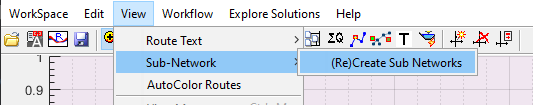

   

   To view this, restart the command again. You will now see a list of items, and sub items.

   

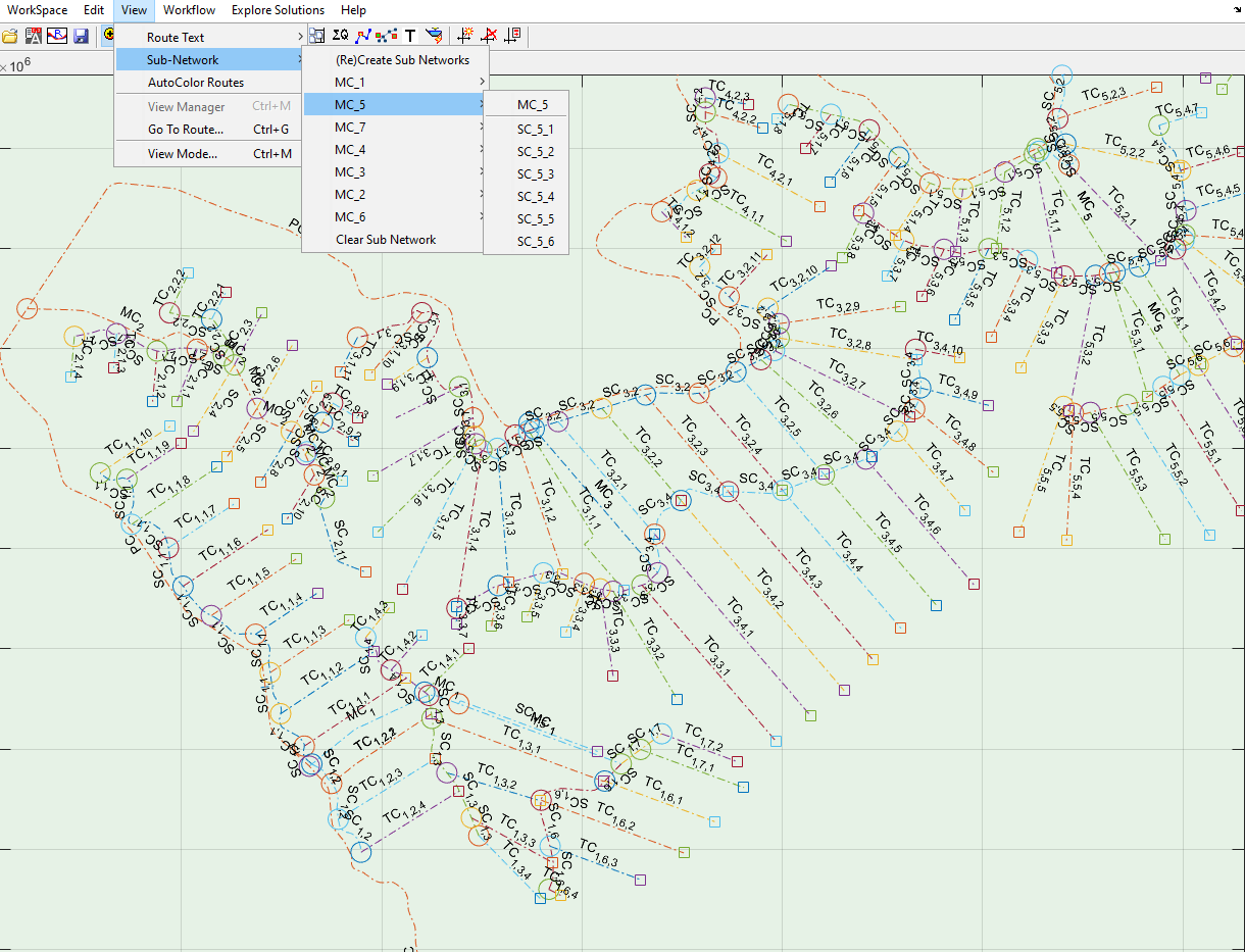
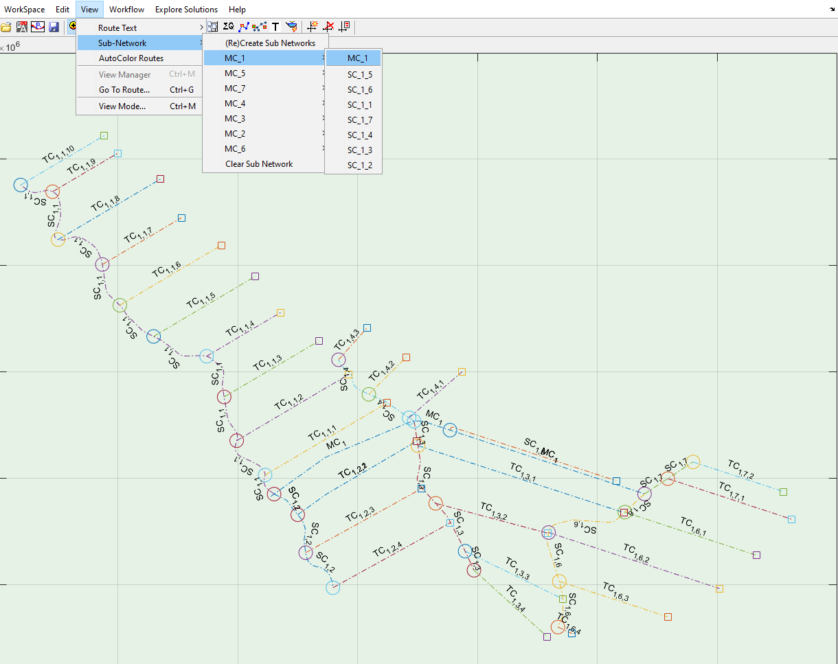
   Click on any one item, only the corresponding routes will be displayed.

   

2. The other method is to use View > Go to Route... menu or Ctrl+G for short. Select the desired route on plan view, and start the command.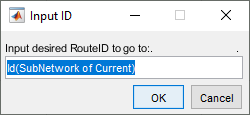

   

   Accept OK on the dialog, and this will retain only relevant canal routes in the view.

You can work on any sub-network, as you would on the entire network. The changes will only affect the network in view.

END.